1. Introduction
An electroencephalogram (EEG) is a graphic representation of neural activity. It is registered from electrodes placed on either inside the brain, over the cortex under the skull or certain locations over the scalp. In this last case, there exists a standardized system, known as 10 – 20, which systematizes the location and identification of the electrodes [
1]. In both cases, each electrode samples mostly the synaptic activity that occurs in the superficial layers of the cortex. The signals obtained from them are normally presented in the time domain, but new EEG devices apply simple signal processing tools to visualize the brain activities in the spatial domain.
EEGs have became a fundamental tool for the diagnosis of many neurological diseases, for example epilepsy and sleep disorders [
2]. It is well known that the EEG is very sensitive to the action of pharmacological substances, especially psychotropic drugs, anesthetics and anticonvulsants [
3,
4].
Usually, clinical interpretations of an EEG record are achieved by associating pathological features with the visual inspection and pattern recognition of the EEG. Even when this traditional analysis is quite useful, the visual inspection of the EEG is subjective and it does not easily allow any systematization. Therefore, it is of utmost importance to provide quantitative methods of analysis that allow the evaluation of the therapeutic efficiency of a particular drug and the clinical evolution of patients.
The quantitative analysis of an EEG record has been based, mainly, on the use of classical techniques of signal processing. Among them, spectral analyses can be highlighted—fast Fourier transform and wavelets—as well other complex analytical techniques [
5,
6]. Recently, some new approaches to the problem of the quantification of the statistical and dynamical characteristics of the EEG series were achieved by using techniques and methods from information theory and nonlinear dynamics [
7,
8]. The starting assumption when these approaches are used is that the EEG records are complex signals whose statistical properties depend on both space and time. Regarding temporal characteristics, EEG signals are chaotic and highly non-stationary. Nevertheless, they can be analytically subdivided into short representative epochs, where the stationary hypothesis is accomplished [
9].
Several works have been devoted to quantifying the therapeutic effects of drugs from the analysis of EEG records by means of quantities arising in the theory of nonlinear systems [
10]. One of these quantities is permutation entropy (PE). Introduced as a statistical measure in the realm of chaotic systems, PE describes complexity through a phase space reconstruction, which takes into account the non-linear behavior of a time series [
11]. In the context of neurophysiology, the PE has been used to measure brain connectivity in epileptic disorders [
12], to characterize epileptic seizures [
13–
15], to measure the effect of anesthetic drugs [
16,
17] and to study complexity in Alzheimer’s disease EEGs [
18], just to mention a few examples. In the same direction, we develop a method based on PE to characterize the changes that occur in EEG records obtained from a patient suffering generalized tonic-clonic seizures. The analyzed EEGs were recorded at different stages of the pharmacological treatment of the patient (with an anti-convulsive drug). Our results show that PE could be a useful tool for neurophysiologists to evaluate, in a quantitative way, the clinical evolution of the patient along the treatment course.
The paper is organized as follows: in Section 2 we provide some basics on PE (or Bandt and Pompe entropy). In Section 3, we describe the main clinical characteristics of the patient, and we report our results. Finally, in Section 4, we address some conclusions.
2. Permutation Entropy
Every dynamical system can be represented by using a symbolic sequence. There are many means of mapping a continuous time series onto a symbolic sequence. A method particularly useful has been developed by Bandt and Pompe in 2002 in the realm of chaotic systems [
11]. In this section, in order to make this work self-contained, we will give the basic ideas underlying the definition of PE. However, the reader could find it useful to consult some works where the main properties and applications of PE in different contexts have been investigated [
19].
To fix the ideas, let us consider a real-valued discrete-time series {Xt}t≥0, and let d ≥ 2 and τ ≥ 1 be two integers. They will be called the embedding dimension and the time delay, respectively. From the original time series, we introduce a d-dimensional vector
:
The superscript T stands for transposition.
There are conditions on
d and
τ in order that the vector
preserves the dynamical properties of the full dynamical system [
20]. Next, the components of the phase space trajectory
are sorted in ascending order. Then, we can define a permutation vector,
, with components given by the position of the sorted values of the component of
. As an example, let us consider the time series
Xt = (1.7, 2.1, 1.5, 1.4, 2.2). Let us take
d = 3 and
τ = 1. The vectors
are (1.7, 2.1, 1.5)
T, (2.1, 1.5, 1.4)
T and (1.5, 1.4, 2.2)
T, and the corresponding permutation vectors are (2, 0, 1)
T, (2, 1, 0)
T and (1, 0, 2)
T. Each one of these vectors represents a pattern (or motif). There are
d! possible patterns. For a sequence large enough compared with
d!, it is possible to calculate the frequencies of occurrence of any of the
d! possible permutation vectors. From these frequencies, we can estimate the Shannon entropy associated with the probability distributions of permutation vectors. Some of the possible patterns may never occur. If we denote the probability of occurrence of the pattern
i-th by
Pi, i ≤ d!, then the (normalized) permutation entropy associated with the time series
Xt is (measured in bits):
The fundamental supposition behind the definition of PE is that the d! possible permutation vectors might not have the same probability of occurrence, and thus, this probability might unveil knowledge about the underlying system.
As was indicated above, an EEG time series has changing statistical properties. Our basic assumption is that PE must show these changes. Therefore, for quantifying these changes, we define a probability distribution of patterns Π’s along the record. The scheme consists of introducing a sliding window that moves along the original signal. For each position of the window, we can evaluate the probability distribution of the patterns for the signal limited by the borders of the window, and so, we can evaluate a time-dependent PE.
Schematically, our method can be described in the following steps:
Step 1: Let us define a sliding window of width ∆ > 0 and position k (which indicates the position of the right side of the window). This window moves along the original signal.
Step 2: For each position of the window, we evaluate the permutations vectors as explained before. We denote this set of patterns by
Step 3: For each value of k and from the estimation of the probability distributions of patterns
, we evaluate the associated PE as a function of the cursor position.
3. Case Study and Results
We apply the scheme described above to the analysis of EEG records obtained from a 20-year-old patient, with an electro-clinical diagnosis of idiopathic generalized epilepsy, at different stages of pharmacological treatment. The patient underwent an initial treatment with a 1200-mg/day dose of carbamazepine. Along this period, the patient suffered an average of ten convulsive crises per week. At a certain moment of the treatment, let us say at time T1, the dose of carbamazepine was reduced to 400 mg/day, and the patient was co-medicated with a dose of 1000 mg/day of valproic acid (VPA). The inclusion of the VPA decreased the number of crises to two per month. This treatment lasted for almost one year.
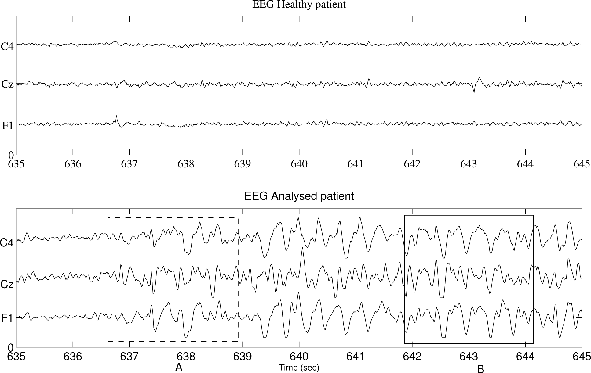
Figure 1 shows some representative electrode traces recorded from a healthy patient (upper panel) and from the patient under study (lower panel) at a time previous to
T1. The EEG was recorded during one hour, with the patient in the basal position, and along the record, no convulsive crisis was observed. The data were hardware filtered between 0.5 and 70 Hz. The sampling rate was 65 Hz (the same conditions are valid for all of the records used in this work). The signal inside the dashed line and continuous line boxes (A and B, respectively) plus clinically relevant information allow the neurophysiologist to characterize the disease. Inside the regions limited by Boxes A and B, different higher voltage discharge patterns in both frontal areas can be observed. Usually, they are associated with epileptiform discharges.
At times previous to T1, between two and three paroxysms per minute were observed. If these, 38% of the paroxysms had a duration not less than 10 seconds, and only 16% had a duration greater than 20 seconds. Most of these paroxysms had a frequency of three spikes per second. The greatest voltages recorded corresponded to the F electrodes. Therefore, it can be concluded that the dysfunction is prominent in the frontal region. A similar analysis of an EEG record obtained one year after the VPA administration shows that the number of paroxysms per minute reduces notably, as well as their duration.
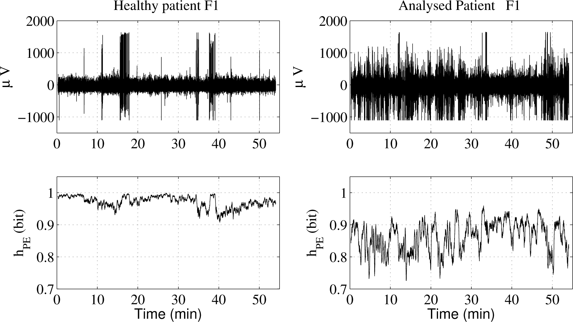
Figure 2 shows the traces corresponding to the F1 electrode and the PE evaluated from this waveform, according to the scheme described in Section 2. The left plots correspond to a healthy patient, and the right plots correspond to the studied patient. The PE was evaluated for an embedding dimension
d = 4 and a time delay
τ = 1. The moving window has a width equal to ∆ = 1000. We chose the value
d = 4 in order to satisfy the condition that the number of values inside the sliding window was markedly greater than
d!. We have checked that our results are not modified by choosing
d = 3. The resulting values of the PE are notably higher for the healthy person than for the analyzed patient. For this, the EEG was recorded before time
T1, that is previous to the administration of VPA.
Previous to the treatment with VPA, the patient had generalized diurnal and nocturnal convulsive crises. After the VPA therapy, the frequency of the crises start reducing notably, until reaching the value of two crises per month. When co-medicated, the crises were of the tonic type, occurring only at night time.
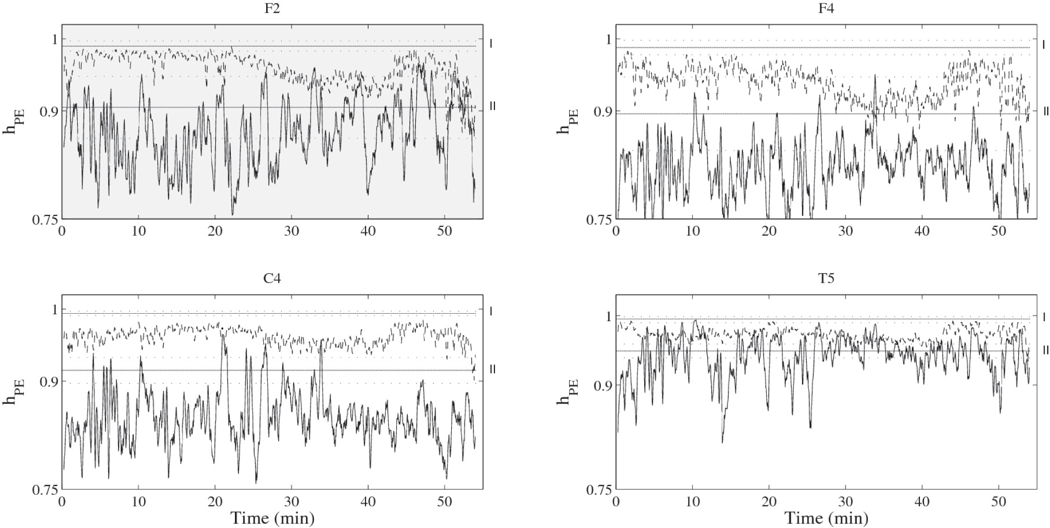
Figure 3 shows PE calculated from some representative electrodes’ signals. The continuous lines are used in the plots calculated from the EEG recorded previously to time
T1 and the dashed lines for one recorded one year after
T1. All of the values corresponding to healthy patients lie inside the band demarcated by the horizontal lines, I and II. The results show a displacement of the values of the entropy
hPE to values corresponding to healthy people. The effect is most notable for the signals recorded from the frontal electrodes. For another case already studied (not reported here), the same behavior is observed.
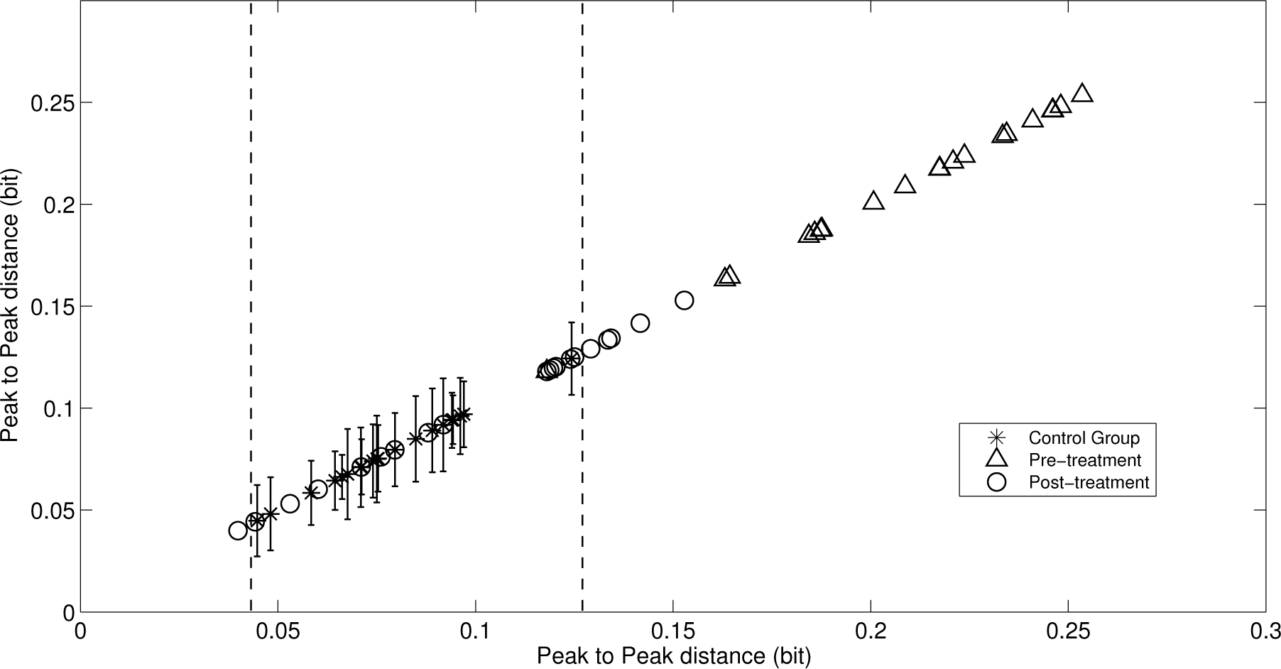
To evaluate the evolution of the patient along the period of co-medication with VPA, we compare the values of PE, calculated from the wave form recorded from each electrode, with the average of the values obtained from a group of 20 healthy patients (control group). We use as the variable to be plotted a range of values of PE defined as the difference among the higher values and the lower values of PE; that is, a peak-to-peak difference. In
Figure 4, we plotted the resulting values. We used the ∇ symbol to indicate the values measured in the patient suffering the epileptic seizures at times previous to
T1 and the ○ symbol for the values measured one year after time
T1. The ∗ symbols represent the average of peak-to-peak values of PE over the 20 healthy patients. Each symbol of different types corresponds to one electrode. Along the VPA treatment, we observe a displacement of the PE values toward the average range of values for healthy patients. In is important to note that every pretreatment value of PE lies outside of the range corresponding to healthy patients. We did a similar evaluation changing the embedding dimension
d, and the same behavior for the values of PE has been observed. In that sense, our results are robust.


