Interactive Data Visualization for the Web by Scott Murray: Book review

Interactive Data Visualization for the Web by Scott Murray
My rating: 4 of 5 stars

This is really a d3.js (Data Driven Documents) book, since the entire book is about using the d3 Javascript library for data visualization. For me, coming in with a background in data analysis but no practical Javascript background, this provided a good overview of many Javascript/web concepts required then the d3 library.

My background in data visualization is R (ggplot and lattice) and Python (Matplotlib). I find Excel too limiting and Matlab inflexible. But what I'm used to are descriptions of visualizations that are then implemented. d3 is different, it makes you specify the form of the visualization and makes you work at a very low level (which is what ggplot and Matplotlib are trying to avoid). But this provides room for great creativity, and learning how to do this is the point of this book.

This book does a good job of introducing enough of the background technologies of Javascript and the web to make d3.js useful. This was always the reason I never got around to actually using Javascript, I never learned all the things you needed to know to make it useful. For example, I now think I understand JSON well enough that I can see using it as a data store for data frames instead of CSV or SQLite or pickles (Python).

I come at this as someone who already does data analysis, but may need more ways of delivering the products of the analysis to others. And this has promise as a means of this delivery through a browser, which is already comfortable for most. And this book does a good job of working both the subject of d3.js and the web ecosystem that it is a part of to get to someplace useful.

Disclaimer: I received a free electronic copy of this book as part of the O'Reilly Blogger Program

View all my reviews at Goodreads.

A recap on work flow, note takers and task organizers

Some experiments I have been doing with workflow over the past semester as introduced on this post back in January. 

1.  Using Pandoc, Markdown, and pweave for class preparation.  

I did the notes for my Logistics and Supply Chain course completely in Markdown.  This included slides for in class presentation, writing homework solutions, and everything else with the class preparation.  I wrote a Makefile that took care of everything.  Basically what it meant is that to create slides for class prep I wrote it as a text file.  It does force some simplicity because there is no ability to tweak a slide or an image.  But that is probably a good thing because it forces efficiency.

One nice advantage of using pweave for homework and exam solutions is that it makes it easy to have multiple versions of an exam.  If I have equations and steps in place, I can change a few parameters, and maybe an assumption or two and I have a new problem with not much extra work.  Also I did a lot of cut and pasting of code.  The code I wrote for presenting in class became the code that I used to solve the homework.  And since I let them see the code (and I also copied over the equations needed to solve the homework) it connected the homework solution to the lectures.  One issue is that so few of my students were competent programmers in any language that the Python code was not all that helpful to them (other than proving that I did indeed solve the problem)  But this was a definite success.

2.  Using Mercurial as a hosted version control system.  

I had to work with a new team on one project I was working on, so the first thing I did was to move the  former post-doc's work into a version control (Mercurial) and put it on a hosted repository (bitbucket).  And we spent a month refactoring the entire thing to separate out the code from the site specific bits (because we were going to apply it to a new location).  The repository meant that we were able to be aggressive in refactoring (yes, I did have to completely through out a day of work at one point because what I was thinking was not going to work.  All I did was wipe my directory and reclone the repository)  The others got into the hang of putting everything in the repository as well.  Now, the comments are not all that good on the part of the post-doc and grad student working with me, and we tended to work in separate areas so it was not true collaborative programming, but it was not bad.

I plan on continuing this over the summer with a few students who are learning agent based modeling together.  The intent is that if all of us are putting our models in the repository, we can ask questions like "why does ___ not work" and we can have their model to look at.  We'll see how that works.

3.  Google Tasks as a task organizer  

This worked out pretty well.  I ended up using Google tasks as a note taker (more on that later)  I was off an on regarding being consistent, but there were periods where I had a lot going on that this to-do list being available on all of my computers, my iphone and ipad was very useful.  Keep doing this.

4.  Tomboy as a notes organizer. 

Note taking sounds like a no-brainer.  Not.  This one pretty much died.  In February Canonical eliminated an API that enabled use of Ubuntu One as a storage place.  So I ended up storing the notes data on Dropbox (so my Windows and Linux machines were synced).  But the iPad app that integrated with Tomboy no longer worked, so if I was using the iPad, the notes were not integrated.  And this pretty much meant I was not using Tomboy notes.  Sometimes I would create a task in Google tasks and create a note if I needed something.  But generally this went unused.

I'm going to try this again.  But since I realize now that having it on my iPad and syncing to my computers is the key to the whole affair, my main focus was on the iPad integration.  So I am looking at Simplenote for the note-taking. It is originally designed for iPhone/iPad, and there are applications on Windows and Linux that integrate with it (and also the Google Chrome browser)

Personal experiments on workflow, note takers and task organizers

This semester I'm undertaking a few experiments in productivity.  Now, most of my work as a professor does involve computers, either developing and implementing models and methodology, preparing course lectures and materials, and communicating, and managing others.  And this spring, I have a fairly challenging schedule from an organizational standpoint.  In addition to the standard course and research projects I am working with a new (to me) graduate student and post-doc, I am running the department senior project course (with the department chair to back me up), and I am involved in one of those long-term career milestones.  So part of this past winter break was spent setting up systems to improve productivity.  Some minor workflow issues.  And some larger ones.

1.  Using Pandoc, Markdown, and pweave for class preparation.  

I long ago decided on Beamer as my preferred method for preparing presentations.  Using LaTeX essentially forces the use of styles instead of fiddling with page layout (or having your styles get overridden without notice) and I can focus on content rather than form.  But there is alot of scaffolding that goes into any LaTeX document.  Enter Markdown.  I already use Markdown with R using knitr, which allows me to keep both the documentation about a method along with its coded implementation and the output of the code in a single document with a syntax that is not that far off what you would naturally do if you had to format a document using plain text (e.g. using Underlining and blank lines to set off headings or '*' to identify emphasized words.)  So Pandoc is a utility that allows me to use Markdown format to generate slides in HTML5 or as PDF files (via Beamer).  And pweave does for Python what knitr and Sweave do for R, combine the documentation of algorithms, the implementation, and the output in a single document where the output will automatically update as the implementation or the input data changes.

So now, I can build slides in Markdown that includes the lecture, the math model, a Python implementation of the math model, and the output of the implementation.  And since Markdown is a lot less complex than LaTeX, hopefully do this faster than I was before.

2.  Using Mercurial as a hosted version control system.  

I was running a project that was based on a simulation being built over a period of years by a post-doc.  However, he was really the only one working on the code.  It was at the point where I wanted to do some side experiments with our model, so I wrote another implementation in Python. (note, using SimPy, it took me two weeks).  But now he has moved on, and I'm still working on the project with another post-doc and grad student. So, since they are new, and we are jointly working on the model to apply it to a new system, I've taken the model from Dropbox (shared folders) to distributed version control, namely Mercurial on Bitbucket.

While Git is the more popular (at least among hipster elite programmers), Mercurial uses commands similar to Subversion (which the post-doc already knew) and tools were readily and obviously available for both Windows and Linux.

I've been using Mercurial and Bitbucket for my own projects including coding and writing papers in LaTeX for a while now, but this is the first project of my own that I have other people working with the same repository.  So I'm training them along the way.

3.  Google Tasks as a task organizer

I've started using Google Tasks. At one point I was using Remember the Milk, but I stopped because it was not integrating well with Google Calendar (which is how I do my scheduling). (RTM put an entry into every calendar day, which means I had to open my calendar to see if the marker was real or empty)

So with Google tasks, I can create a task in the Google Calendar sidebar, in the sidebar of Google mail, or there is an iOS app (GoTasks). The interface is not as pretty as Remember the Milk, but it works better with my Calendar. And the iOS version is not crippled (RTM is limited to one update a day on the free version).  The main criteria here was the fact that it worked on all of my computers (I use Windows, Mac OS X, and Linux in different settings) as well as my iPhone and iPad (because I often go to meetings and trips with just my iPad and not my laptop)

4.  Tomboy as a notes organizer.

This past fall I was working with an undergraduate who learned the use of MS OneNote while a summer associate with McKinsey and I was impressed about how well he could organize and use these free form notes. I had been using Google Docs to do this, but the need to get on the internet, fire up the browser, and then work was sometimes too much, and it was hard to organize.

Tomboy is a fairly lightweight application.  It provides a formattable and linkable text area, but not as heavy as most desktop applications.  Tomboy can also work with a cloud storage account such as Dropbox or Ubuntu One to keep the data in the cloud, to be synced whenever your computer is on-line.  So now, I have set up a notes folder for the senior design project, with subfolders for each team, a folder for my major research project (with the grad student and post-doc), and my other project.  And I know have collections of short notes that are each dated, identified with keywords, and linked to each other as much as needed.  And I can access and edit them from each of my computers, my iPhone and iPad.

So, here is the great experiment, cobbled together in the midst of all the other work and writing I was doing over the winter break.  And next week is when the fun starts.

A free, public domain recording of the Goldberg Variations performed by Kimiko Ishizaka

Last Monday was marked on my calendar as the release of The Open Goldberg Variations performed by Kimiko Ishizaka.  Why was that special?  It was the release of a crowd-funded professionally performed, recorded, and produced recording and score of Bach's Goldberg Variations into the public domain.  It is a throwback to the old system of patronage for individuals supporting artists and their works.

Arguably, the enduring contribution of this is the release into the public domain of both the score as well as the MuseScore source file.  As programmers know, the release of the source file in an open format with an open source implementation means that this will be available for re-formatting, re-publication, and combining with other similarly licensed works forever.  It also means that the score has been examined, not only by those who were directly funded by the project, but by anyone who had the inclination and interest to participate in the project over the past year.  The process was open for examination not only for correctness, but also feedback and ideas.  No small matter in piece that was meant for a double manual (keyboards) of a harpsichord instead of the single keyboard of a piano.  While the notes may be by J. S. Bach, how it is presented and arranged so a pianist can play it when the physical layout of the instrument is different then intended matters.  The challenges of this have lead to improvements on the open source MuseScore composition and notation program (and I for one am waiting for the release that includes these improvements to come out). Aaron Copland (and others) have stated that music is a collaboration between composer, performer and audience.  In many cases, the third is often diminished, reduced to paying for tickets, recordings, and donations.  But here, the fact that the audience could contribute was taken seriously.

I'm already familiar with the piece from the 1955 Glenn Gould recording.  And since the release of The Open Goldberg Variations I have had this playing in the background continuously while working.  Which, come to think of it, is not much different than the original purpose of the piece, to provide something to be played by Johann Goldberg to play for the Russian Count Kaiserling to cheer him up during his insomnia. And last night when everyone else in the household went to bed, I stayed up to listen to this with a copy of the public domain score (from MuseScore.com) in front of me.

Looking at the score, one obvious note is the utter absence of dynamics and tempo markings.  Which leaves considerable room for interpretation.  The range of the 30 variations (plus the base Aria and final Area da Capoe è Fine) allows the pianist to show her range, and Ishizaka provides something to hear.  As expected, she does not make the same choices as Gould.   And she does not seem to be in as much of a hurry as Gould was. And the recording became a delight as she worked her way through the variation, each with its own feel, even with each repeat.

Here in Pittsburgh, I've had the please of being a part of an experiment by the Pittsburgh Symphony to involve a part of the audience as part of its blog.  Because for the audience to take its place in the three aspects of composer/performer/audience there should be more response than only our monetary support of institutions, but to contribute to criticism and direction of the art.  And this project pushed that in a way not common today.

Is this model sustainable?  Since it was funded through Kickstarter, the professionals involved did indeed get paid.  Looking at Kimiko Ishizaka's website, she seems to have a nice international concert schedule with many recent and future bookings that are easily attributable to her participation in this project and the Well Tempered Clavier (which is a potential following project).  Similar to programmers making a name and reputation for themselves by contributing to open source projects, Ishizaka seems to be taking advantage of the additional exposure coming from her participation.  And similarly to open source, the observation is that professional quality work on well run and managed projects leads to high quality products and opens leads on future work.

If you have any interest in listening to classical music, I highly recommend downloading the recording (MP3 and FLAC available at Soundcloud below).  If you want to follow along with the score, or if you are thinking of actually playing this yourself, get the score from MuseScore.com.

Getting SageTeX to work on Ubuntu

Since I'm using Sage more, I'm trying to get SageTeX working, so I can embed Sage into LaTeX documents (i.e. have a report on the methods integrated with the code that implements the methods and generates the results. Search for 'Literate Programming' or 'Sweave' for many references on this)

On Ubuntu, after I copied SageTeX files to my local LaTeX configuration directory (as per instructions in the Sage Installation Guide, I still got errors when trying to build the example documents

Traceback (most recent call last):
File "st_example.py", line 7, in
_st_.inline(_sage_const_0 , number_of_partitions(_sage_const_5 ))
File "/home/lluang/Apps/sage-4.7.2/local/lib/python2.6/site-packages/sagetex.py", line 86, in inline
'}{{%\n' + s.rstrip() + '}{}{}{}{}}\n')
File "element.pyx", line 331, in sage.structure.element.Element.__getattr__ (sage/structure/element.c:2868)
File "parent.pyx", line 327, in sage.structure.parent.getattr_from_other_class (sage/structure/parent.c:3193)
AttributeError: 'sage.rings.integer.Integer' object has no attribute 'rstrip'

**** Running Sage on st_example.sage failed! Fix st_example.tex and try again.


So what happened? Apparently, one of the Ubuntu texlive packages (specifically texlive-latex-extra) includes an outdated version of the sagetex.sty file while what is needed is one tailored to the current version of Sage (and included in the Sage distribution). While I have the correct version in a local directory, there is a precedence issue when multiple LaTeX style files are present. Since I don't have the inclination to figure out the issue, I found the location of the wrong sagetex.sty file, and deleted the entire directory (/usr/share/texmf-texlive/tex/latex/sagetex). Now, SageTeX works, and I can start writing papers using Sage/Python, just like I do using Sweave for R.

Teaching Notes: Simulation Fall 2011 and using Simpy and Sage

This was my first semester teaching a graduate level (research focus) simulation course. The department has not had this course in quite some time. There is a master's level graduate course taught by an adjunct professor that focuses on simulation modeling (i.e. building the models, with an explicit de-emphasis on analysis). This course, in stark contrast was to focus on the analytical side of simulation with a de-emphasis on model building (i.e. the models used would be considerably simpler then would be expected in the other course, including the project).

The other goal was to learn a new simulation library. I wanted to learn to use Simpy simulation library as it is used by researchers associated with a computational research center at my school. I was using this within Sage, a mathematical programming environment. Sage in its notebook mode was how I was going to present the material, as it allows for mixing formated text as well as showing the results of calculations, graphing of results, etc. I wanted to test live generating of graphs and output of random simulations, to demonstrate the effects of randomness throughout. I let each student choose a simulation platform. The standard here was Arena. The other options were simulation libraries targeted at various simulation languages such as Simpy (Python), SSJ (Java), Simlib (with the Law and Kelton books for C/Fortran) or Omnet++ (C++).

The students were a mix of engineering PhD/MS students and students in the MBA/MS-Industrial Engineering (IE) program. Note that there is some selection here, as everyone is fully aware that the other graduate simulation course would be offered in the spring. Actually, one of the MSIE students had previously taken that course. Most students used Arena. One used Simpy and one used Matlab (i.e. roll his own)

Some notes

1. Teaching MBA/MSIE students was fun. If this is what teaching MBA students is like, I'm all for it. These students were attentive, frequently asked very insightful questions, eager to learn the material and implement it, and were quite appreciative of the analytical focus of this course. A few of them mentioned that since they were interviewing for jobs, topics covered came up in their interviews (clearly, these were quantitatively oriented MBAs). One issue was during projects, as one of the PhD student projects was based on what he was exploring as a PhD thesis, I had to explicitly state that there were different standards for projects.
2. An analytically focused simulation course was the right idea. The MBA/MSIE students liked it and appreciated the difference, including the one who took the other simulation course previously. Focusing on the use of simulation instead of the building of simulation models put the emphasis on the use of simulations for decision making (which allowed the MBA students to bring in what they knew from other courses with them). And for the PhD students, implementing analytical methods gave them an understanding of the field. And a decent part of one PhD dissertation is going to come out of the course.
   
3. Simpy - I liked using Simpy. I found it fairly easy to pick up once I started putting some time into it. One issue was the general flexibility of programming language simulation libraries compared to commercial packages. My general pattern for solving a homework problem was to (i) take code from a similar problem, (ii) (re)write a class to incorporate the differences, (iii) write data collection code (iv) analyze results. But what happened to those who used Arena was they could not get modules to do what they wanted, and developing data recording procedures for an arbitrary performance measure and getting the per-replication output in Arena could be a daunting task. So what took me 20-30 minutes sometimes took the students hours.
4. Sage - The Sage notebook view was very useful since it allowed the mix of formatted text (like a Powerpoint slide would have), along with live calculations. I used this along with simulations to demonstrate the effects of random variables and to show how various formulas and algorithms are actually implemented. (the descriptions in books and articles skip implementation details) Having the description alongside implementation made sense. When asked, the students preferred this version over the alternative of me drawing on the board (which I also did on occasion) and definitely better then Slides (with the benefit that slides give of having distributable lecture notes). One other benefit was I had to make sure I understood everything, because I would implement every procedure discussed in code including charting before giving the lecture, since the implementation was part of the lecture. There was a similar downside of the students not being able to efficiently replicate the analysis, as they were mostly using Excel spreadsheets for analysis and it was sometimes time-consuming to do tasks that programming made quick.
5. Sage data analysis. Sage uses the Matplotlib library for data display and graphics. It is reasonable capable, and I have more flexibility than say R. But the tighter integration with the data analysis techniques already built into R make R a better platform when it comes down to it. Sage/Matplotlib has the advantage that modeling can be done in Sage/Python, allowing for all in one tool. (R can be accessible from within Sage, but it is not straightforward once you get past the R core functions)
   

Conclusions

1. An analytically focused course works, even with non-PhD students (who were admittedly self-selected)
2. The Sage notebook view is useful for teaching purposes. Formatted text, LaTeX for equations. Sage's ability for typesetting symbolic math and putting descriptions as well as implementation side by side was useful. Especially in stochastic settings where people do not have well developed intuition on the effects of stochasticity. I like this as a teaching environment. Unfortunately, this seems to be difficulty to teach people how to install it so I'm on my own here :-(
   
3. One issue is having people in the same class using commercial simulation packages and programming languages. It is very easy to create a problem that is unexpectedly difficult in a commercial simulation package (and I have no reason to believe that it is a particular failing of Arena). The lack of flexibility in modeling, data collection and analysis makes it easy to get a student in trouble. And I am convinced that this occurs in practice once you leave the core domain the packages were designed for. (I get direct personal contact with representatives from the companies behind a couple of the packages so I get to have this discussion directly with them.)

Installing pyspatialite

Goal: To use spatial databases to perform operations such as centroid, nearest point, and distances to generate a table of distances along a road network from area to area, using the nearest node to the centroid of an area to represent the area.

Backup plan: Create a list of nearest node to centroid of areas. Use some code I have previously written in R to implement Dijkstra's algorithm.

Preferred method: Programmatically access Spatialite and perform all functions in spatialite.

Barrier: Most distributions of SQLite (including the sqlite3 library included in Python) do not enable loading of extentions.

Solution: Install Python module pyspatialite.

Installing pyspatialite is done through easy_install: sudo python setup.py install

The documentation mentions that you need geos and proj libraries installed. What it does not tell you is that you need the development versions (which include header files) of these libraries, as well as the Python headers. After installing the developmental files, then you can install pyspatialite.

Creating spatial data files

At my school, there is a class on Geographic Information Systems (GIS). When you complete the class, you now know how to analyze data using ArcGIS. But you do not know how to create the data files you used. And you do not know how to do anything that ESRI did not include in ArcGIS. As a researcher, I find that unacceptable. This year, there is a senior project team including someone who has taken this class doing a project with the local chapter of the Red Cross that will involve using spatial data. But since they cannot create a spatial file, I will create the data sets that they will use to populate their models. If I am going to do something, I may as well learn something along the way. Those somethings are Spatialite and Google Maps API for geocoding.

Step 1. Given a list of addresses, find their latitude and longitude. The official way to do this is to get the TIGER line files of street maps. These encode each block by name and the end points of addresses for each block along with their geospatial coordinates. Then you can interpolate. The more pragmatic way of doing this is to find someone who has already processed the TIGER line files and created an API or other interface to work with them. There are many that will then create Keyhole Markup Language (KML) files as output, and I have used one before.

The way I will do it is to use the Google Maps API. There is a Python package called googlemaps that will find lat/long given a properly formulated address. (note: long is a keyword in Python, so we use lng for longitude)

from googlemaps import GoogleMaps

def getlatlong(gmaps, streetaddress, city, state, zipcode):

address = streetaddress + " "+ city + ", "+ state +" "+ zipcode

lat, lng = gmaps.address_to_latlng(address)

return lat, lng

# get api_key from http://code.google.com/apis/maps/signup.html

api_key = "APIKEY"

gmaps = GoogleMaps(api_key)

. . .

lat, lng = getlatlong(gmaps, streetaddress, city, state, zipcode)

Step 2. Create an Spatialite database. Spatialite is the SQLite database with extensions for Simple Features for SQL, i.e. a relational database that allows for queries on geometric objects. The other options are Oracle Spatial, DB2 Spatial, PostGIS and MS Server with spatial extensions. There are also spatial extensions to MySQL, but they do not meet the SFSQL standard, and they are simplistically implemented (which would lead to many errors if you actually needed correct answers instead of approximations.) Of these, Spatialite does not require an administrator and contains its data in a single file, both of which simplify their use. To use Spatialite, the PROJ and GEOS libraries should already be on your machine. (see Spatialite installation instructions)

To create a database, use spatialite the same way as you would have used sqlite. But after creating the database, load init_spatialite.sql This SQL file loads some required tables. Sometimes, Spatialite will create the tables on its own, but sometimes not (especially if the database was originally an SQLite database).

Next, load the data (using any of a variety of different methods for SQLite databases.) Given address data, determine lat/long and enter each of them into their own fields. (you probably have to create these fields after importing the address data.

Step 3. Create the geometric representation of the data. What makes data spatial is the connection of a geometric representation of the data and the information about the spatial object. Before you do this, it would help to look at other datasets you are using. Spatial data is usually distributed as ESRI Shapefiles. Each Shapefile is actually a collection of files that include the polygons of the geographic objects, the data associated with those polygons, and a projection that describes how to make a representation of a surface of a sphere into the two dimensions of the computer screen (or piece of paper). The projection of a shapefile is usually found in a *.prj file in the same directory as the *.shp file. Most GIS viewers allow you to look at the shapefile properties from within the GIS viewer. The value needed is an SRID, usually a 4-digit number (sometimes 5). From here, a set of spatial queries are run from within Spatialite to add the geometry to the database. See prior post on loading lat/long data in Spatialite. When these spatial functions/queries are run, Spatialite will perform a series of operations that use the information in tables loaded by the init_spatialite.sql to generate the geometry representation or convert representations between projections. At this point, the data is now spatially enabled.

Step 4. View/Export. At this point, only a few GIS viewers can use Spatialite databased directly. One is QGIS. So after performing any wanted spatial queries or other operations you should export the data to another format, such as Shapefiles. The OGR/GDAL tools of the Geospatial Data Abstraction Library are able to do this. Within Spatialite you can use the .dumpshp function to create a shapefile.

The format of .dumpshp is

.dumpshp table Geometry sitelocations CP1252 POINT

table is the TABLE to be exported. I think this could have been a VIEW as well. Geometry is the name of the field within the table that has the geometric representation. Note that Spatialite stores this as a BLOB object. sitelocations is the name of the shapefile to be created. CP1252 is the name of a character set. Presumably there are others, but I have been using CP1252 for now. POINT is the spatial data type. Other types include LINESTRING, POLYGON, and MULTIPOINT.

What would be very useful right now is if I could automate steps 3 and 4 so I could run them from within Python instead of doing them inside Spatialite. However, this only works if SQLite was compiled with the ability to load extensions. Most distributers do not do so. One workaround is to install the pysqlite2 extension and compile it so that it can load extensions (as opposed to using the sqlite3 extension that is included in Python).

Loading Lat/Long data into Spatialite

The task: Load spreadsheets with Longitude and Latitude data into a spatial format. Preferably in a way that can be done by people who are not good programmers but can follow directions to use command line tools.

Initial data: Spreadsheets with addresses and Longitude and Latitude. Note: this can be created using the Google Maps API accessed through various programming interfaces.

Tools: Spatialite and SQLite Manager (Firefox plug-in)

Steps:

1. Save spreadsheet as a comma separated format
2. Import into SQLite using SQLite Manager plug in
3. Open Spatialite using command line interface.
4. Add the geometry to the table using: SELECT AddGeometryColumn('addresstable', 'the_geom', 4326, 'POINT', 2);
5. Note that 'addresstable' is the table within the database that contains the long/lat data. 'the_geom' will be the new field that contains the spatial data. 4326 represents the SRID for the projection to be used (in this case WGS 84). 'POINT' is the spatial data type. 2 indicates this is in a 2-D space.
6. Calculate and insert the spatial data using: UPDATE 'addresstable' SET the_geom = GeomFromText('POINT('||Longitude||' '||Latitude||')', 4326);
7. Longitude and Latitude are the field names containing the longitude and latitude data in the table. The names do not matter. But they order does. And they are separated by a single space.
8. Method is taken from PostGIS in Action by Obe and Hsu. Spatialite function names are similar to PostGIS function names. In many (but not all) cases, the 'ST_' is removed from the beginning of the function name. Note that for the exceptions, the Spatialite documentation references two function names, one without 'ST_' and one with.

WinBUGS and JAGS differences

One of my graduate students and I have been working on input modeling in a setting where the amount of historical data can range from a lot to almost no (i.e. 0, 1, 2) occurrences. So both of us have been learning Bayesian methods and developing means to work with our setting. Part of this involves working with the standard tools and building blocks for Bayesian methods, in particular Monte Carlo Markov Chains (MCMC). To implement these methods, you can program your own, or use some standard modeling frameworks. Some of these frameworks are essentially programming libraries. But the primary ones are Bayesian inference Using Gibbs Sampling (BUGS) derivatives. There are two families: WinBUGS/OpenBUGS and JAGS.

WinBUGS is the direct successor to BUGS, with OpenBUGS being the open source next generation. BUGS is both a software package as well as a model specification language for MCMC models. One issue with WinBUGS/OpenBUGS is that it is written in Component Pascal. WinBUGS depended on the BlackBox component builder, which is only available in MS Windows (as does OpenBUGS, but OpenBUGS is essentially the open source next generation of WinBUGS once it is done). JAGS is an opensource implementation of the BUGS model specification and command language and is written in C++ on top of some open source libraries. JAGS exists specifically because of the inability to port WinBUGS. A review of the literature shows that WinBUGS/JAGS/various other libraries, all have areas of strength and weakness. Research groups working extensively with Bayesian methods use all of the them at various times.

But, this is our first project. So one thing we did was to examine three frameworks while we were learning Bayesian methods. I primarily used JAGS, one graduate student worked with WinBUGS, a third graduate student (the strongest programmer) used MCMCpack (an R package).

Our intent was to use either WinBUGS or JAGS when we actually implemented our methods on real data, so the question was which to use. Some obvious differences that came up.

1. When running using R, the RWinBUGS interface opens the WinBUGS application to run BUGS model. We anticipate having to run this on ~50 separate data sets a day as part of our methodologies. This time of interface is unstable (both theoretically, and practically as my student's computer ends up hanging a lot)
2. WinBUGS is a lot more particular about the BUGS model specification. Or, since the WinBUGS people are the ones who developed the BUGS model specification, it is probably better to say that JAGS is much more forgiving. Some gotchas that came up included:

• When specifying distributions, parameters in WinBUGS could not be expressions. Only single variables. I.e. something like (num1*num2) is not allowed. So we have to perform all computations, then specify the distribution separately. JAGS allows passing an expression as a parameter.
  
• WinBUGS does not have an exponent operator (either '^' or '**') JAGS does. Since one parameter that is important and common is 1/variance, this is very useful when the data is expressed in terms of standard deviation. We have to use expressions like (num1*num1) all over the place.
• JAGS from R is seamless (R2jags, rjags). You call JAGS, and it returns without opening any IDEs. You can see the JAGS output in the terminal, but JAGS runs in command line, then is done. No IDE left to close. (R2jags was designed to work the same way as RWinBUGS, but I think it is much more elegant)
• The JAGS documentation includes some more differences, but we have not hit those yet.

So, for this project, given that we have a certain amount of risk based on the fact that we are figuring out Bayesian methods and MCMC along the way, we're going to go with JAGS as our engine. Someday we'll get better at using WinBUGS/OpenBUGS and MCMCpack, but not today.

Book Review: Beginning Databases with PostgreSQL: From Novice to Professional by Neil Matthew

Originally at Goodreads

Beginning Databases with PostgreSQL: From Novice to Professional, Second Edition by Neil Matthew

My review

rating: 5 of 5 stars
This has proven to be a very good book. I'm not a database expert, but I happen to need PostgreSQL because I am working on a project that involves GIS, and PostGIS turns out to be a very appropriate tool for what I am doing. This book got me started and has helped me through the importing of data, understanding basic functions, and incorporating PostgreSQL into my programs (I use a combination of R, Python/Jython and Java. The book does not talk about them all, but what is in there carries over pretty well.) I've also used this to use BIRT and Openoffice.org to link my PostgreSQL databases. Again, it is not spelled out, but what was in here brought me well along the way to making it work.


View all my reviews.

Book Review: Applied Spatial Data Analysis with R by Bivand, Pebsma, and Gomez-Rubio

Originally posted to Goodreads. Applied Spatial Data Analysis with R by Roger S. Bivand

My review

rating: 5 of 5 stars
Applied Spatial Data Analysis with R (ASDAR) is written by the same people who wrote and maintain the spatial sp class in R. The book is not a statistician's text on mathematical geo-statistics, rather is focuses on taking geospatial (e.g. GIS) data and applying analysis within R. Not being a statistician, I used the book to learn how to manipulate geospatial data for my own analytical purposes. The mark of a good technical book, not only did I learn about how to work with the standard geospatial data types, I was able to implement analyses using the material in the book.


The book has three parts. First is an introduction to spatial data. Much of it is orienting the reader to the vocabulary of geospatial data such as point, line, polygon, grid, coordinate system, projection. It also motivates why using R for spatial analysis. (The other options would be within a GIS such as GRASS or ARCInfo, custom functions using C++ or Java, or Python, which has been incorporated into many GIS environments). In particular, it looks at the many packages and analysis built up that uses the sp package and data structure, allowing many developed analytical methods to be used together to build a complex analysis. (this is similar to my purpose, taking advantage of the fact that R provides a standard entry point to several computational toolkits that I use.)


The second part discusses accessing and using geospatial data in R, which fulfilled my purpose. It is detailed documentation on the various spatial classes and the methods that are applicable. There are descriptions and examples of how to visually display geospatial data. The chapter on data import and export covers GDAL/OGR, coordinate reference systems, projections and transformations, and what you would need to work with formats such as shapefiles, PostGIS, KML, image files such as tiff files and Google Earth overlays (PNG), or directly with GRASS, TerraLib, or Python interfaces with ArcGIS, RPyGeo.


The last part is on implementing geostatistical methods such as for pattern analysis, geostatistics, areal analysis (geographic aggregation), or epidemiology. I cannot comment too much on this as this is not an area that I have expertise, but the methods look both adequate as well as practical to use.


While the intended audience of this book are statisticians working with geospatial data, I would also recommend this to those who do data analysis or modeling with geospatial data. Most of the analytical texts I've seen discuss algorithms. This text gets into the practicalities of working with real data formats and real data issues that are the inevitable first step in a project. And it does so at a more analytical level then the point and click interface instructions that are enabled by standard GIS systems alone.


View all my reviews.

Using shp2pgsql to import Shapefiles to PostGIS

I covered some of this in a previous post on Converting Lat/Long data to PostGIS. But now my problem is to import Shapefiles into PostGIS.

First, why do this. While Shapefiles are good for distributing and looking at data, it is difficult to do any analysis. To do anything, you end up using OGR/GDAL to examine the shapefile and then do something with it. PostGIS takes the spatial and data components of the Shapefile and exposes them in database format, allowing anything that can be done with a database to be done with the Shapefile. In addition, it enables Simple Features for SQL which allows for using set operations on geographic objects (as opposed to only sets). Think of all the Venn diagram pictures back in High School. And other spatial operations that may come to mind when dealing with points, lines and shapes.

The key, of course, is to get the PostGIS database started. So, first, within PostgreSQL, create a database

CREATE DATABASE PA;

Next, load PostGIS onto the database. The first step is to load PL/PGSQL

CREATE LANGUAGE plpgsql;

Next, within the database, load the lwpostgis.sql and spatial_ref_sys.sql into the database. I used the pgAdmin III GUI.

Next, use the shp2pgsql tool The format is:

shp2pgsql [] > .sql

This should be run from the directory with the .shp file. refers to the name of the shapefile. is the name of the table to be created within the database. You can also enter this in schema.tablename form if you want. database name is the name of the database on the local server that it is being entered into. Usual practice is to pipe this to an SQL file that will be read in later (with all the necessary permissions. For option, the common one is to enter the -s of the EPSG (if known).

So, for example, using the NHPN shapefile for Pennsylvania (FIPS: 42), which is to be imported into a database named PACities, in the 'public' schema as the table 'NHPN' with the projection NAG 83 (ft) (Pennsyvania South) EPSG=2272, I get:

shp2pgsql -s 2272 S42NHPN public.NHPN PACities > nhpnImport.sql

And now it is in.

Book Review: Desktop GIS: Mapping the Planet with Open Source by Gary Sherman

Desktop GIS: Mapping the Planet with Open Source by Gary Sherman

My review

rating: 4 of 5 stars
Desktop GIS covers Open Source software for use as a Geographic Information Systems (GIS). In particular, it covers the following programs and libraries:

- Quantum GIS
- uDig
- GRASS(and its Java front end JGrass http://www.jgrass.org)
- PROJ.4
- GDAL/OGR
- PostGIS
- FWTools
- GMT

At the beginning of the book, the author outlines three classes of users. A casual user who only needs to look at data found from elsewhere, an intermediate user who visualizes but also creates or converts data, and an advanced user who has the need to do spatial analysis. To cover all of these is an ambitious goal, which is further diluted by the authors felt need to cover the entirety of open source mapping in one book.

What the author does well is to identify tools, and explains what can do what with enough to get you started. So Quantum GIS and uDig are the viewers, able to read almost any GIS format (in particular the readily-available ESRI Shapefiles as well as PostGIS). GDAL and OGR that can convert anything to anything (including delimited text. These are often distributed as FWTools). PROJ.4 that converts projections from one to another (and is embedded in everything). PostGIS which is the spatial database that enables spatial analysis. And GRASS, which is the full-fledged can-do-everything-but-is-hard-to-learn tool. And then some random programs that either do something completely different (e.g. OSSIM, which is an imagery analysis tool) or can make a picture of a map with lots of options (e.g. GMT).

What he provides are the basics for the casual or intermediate user. The advanced GIS analyst would only have a taste of what GRASS can do, but would not know what can be done with it. Similarly, while the intermediate user will get a sense of what PostGIS can do, the lack of space to cover spatial extensions to SQL supported by PostGIS loses its value to the advanced user. What could have made this book better was more focus. If the author was compelled to have a survey of all open source mapping, it may have gone into an appendix with a few paragraphs for each of the miscellaneous tools. But for the book, one good focus would have been the GIS stack comprising of data storage, data analysis and data viewing. Basically the open source counterpart to the ArcGIS/Oracle with Spatial Extensions. And everything that does not play a role in the stack, gets pushed into the appendix.

What could have been done? The book tended to be organized by tool. But once past the casual user, almost all tasks required multiple tools. I would have gone:

1. Viewing data (raster, vector, introduction to QGIS, uDig, GRASS)
2. Converting data/data formats (GDAL/OGR, Maybe PROJ.4)
3. Creating/Editing data (digitizing, importing)
4. Spatial databases (PostGIS)
5. Geoprocessing/spatial analysis - GRASS, PostGIS, R-spatstats
6. Tools integration (QGIS/uDig with GRASS/PostGIS)
7. Scripting
8. Customization

and everything that did not fall into this gets a page in an appendix.

Knowing where to start is a big help. Most of the websites either focus on one product, or try to teach everything as being equally important. Gary Sherman at least identifies the main building blocks. (QGIS or uDig, GDAL/OGR/PROJ.4, PostGIS, GRASS) and gives enough to get started. And this can be very helpful, so at least the starting analyst knows where to start.

What would be next? For the person still working within the GIS stack (as opposed to a completely different topic, like imagery analysis which is OSSIM's territory) there are a few obvious topics.

1. PostGIS - Spatial databases with SQL. Maybe even connections with ArcGIS. Even a short (10 pg) appendix would have done wonders here.
2. GRASS - The author devotes an additional appendix to this. But to do this right, you probably need to refer to Open Source GIS: A GRASS GIS Approach
3. R spatial statistics packages. Applied Spatial Data Analysis with R would cover this.

Mostly, a good book to get started in GIS using Open Source tools. Casual users would be well served. Intermediate users would get started and can find the rest using the internet. Advanced users are going to miss alot (to the point they don't even realize that these tools were a worthy alternative).



View all my reviews at Goodreads.

Loading lat/long data into PostGIS

Base scenario. I have a datatable with longitude and latitude data that I want to look at using spatial tools. And I have shape files for the metropolitan area that I want to use them with. So, in other words I have the following.

1. ESRI shapefiles
2. Data table with latitude and longitude

The plan is to load the data table into PostGIS, then I can pull them into a GIS system like uDig or Quantum GIS or various ESRI products. Because PostGIS can do transforms, but ESRI shapefiles are what they are, the procedure is as follows:

1. Identify SRID (spatial reference ID) for the ESRI shapefiles. This should include units (feet, meters, or degrees)
2. Identify a corresponding SRID that used lat long degrees
3. Load data table into PostGIS
4. Add geometry (points) data to datatable, including transformation from degrees to feet.
5. Optional: export PostGIS to ESRI Shapefile if needed.

1. Identify SRID (spatial reference ID) for the ESRI shapefiles. This should include units (feet, meters, or degrees)

Shapefiles usually come as a set of files inside a directory. When they come from an official source, one of these should be a *.prj file. This is an example of one

PROJCS["NAD_1983_StatePlane_Pennsylvania_South_FIPS_3702_Feet",
GEOGCS["GCS_North_American_1983",
DATUM["D_North_American_1983", SPHEROID["GRS_1980",6378137.0,298.257222101]],
PRIMEM["Greenwich",0.0],
UNIT["Degree",0.0174532925199433]], PROJECTION["Lambert_Conformal_Conic"], PARAMETER["False_Easting",1968500.0],
PARAMETER["False_Northing",0.0],
PARAMETER["Central_Meridian",-77.75],
PARAMETER["Standard_Parallel_1",39.93333333333333],
PARAMETER["Standard_Parallel_2",40.96666666666667],
PARAMETER["Latitude_Of_Origin",39.33333333333334],
UNIT["Foot_US",0.3048006096012192]]

The first line identifies the projection, using something that should approach a WKT ("Well Known Text") name of a projection. In PostGIS, when the PostgreSQL database was geographically enabled, a table "spatial_ref_sys" was created that has a list of all SRID with names. Searching on this table should reveal a projection that has a name very similar to this one. That will define the target SRID for the whole project. The quick way to do this is to write a query:

SELECT srid, auth_name, auth_srid, srtext, proj4text
FROM spatial_ref_sys
WHERE srtext LIKE '%Pennsylvania%'
ORDER BY srtext;

In this case, we find:

2272; "PROJCS["NAD83 / Pennsylvania South (ftUS)", GEOGCS["NAD83", DATUM["North_American_Datum_1983",SPHEROID["GRS 1980", 6378137,298.257222101, AUTHORITY["EPSG","7019"]],

Note that in this case the key parts were NAD83, Pennsylvania South, and ft.

2. Identify a corresponding SRID that used long lat degrees
Another search through the "spatial_ref_sys" table finds only projections that are associated with feet or meters. So a broader search should be used to get


SELECT srid, auth_name, auth_srid, srtext, proj4text
FROM spatial_ref_sys
WHERE srtext LIKE '%NAD83%'
ORDER BY srtext;

This eventually reveals one projection that

4269;"GEOGCS["NAD83",DATUM["North_American_Datum_1983",SPHEROID["GRS 1980",6378137,298.257222101,AUTHORITY["EPSG","7019"]], AUTHORITY["EPSG","6269"]], PRIMEM["Greenwich",0,AUTHORITY["EPSG","8901"]], UNIT["degree",0.01745329251994328, AUTHORITY["EPSG","9122"]], AUTHORITY["EPSG","4269"]]"

The key here is that the 'UNIT' is "degree" as opposed to "Survey feet" or "Meters".

3. Load data table into PostGIS

First, by this point the PostgreSQL database was created using a template that has PostGIS enabled. I created an SQL file with all the Create Table commands ahead of time. They look like this:

CREATE TABLE table2004
(
case_no character(7) NOT NULL,
week integer,
"month" character(3),
eventdate date,
bg_lat numeric(12,6),
bg_long numeric(12,6),
serial2004 serial NOT NULL,
CONSTRAINT table2004_pk PRIMARY KEY (serial2004)
)
WITH (OIDS=TRUE);
ALTER TABLE table2004 OWNER TO userid;

Key point is that I need something an integer field that is a primary key, or at some points indexing becomes a problem. So I made a serial field to be an index (because my case_no field is a text field so was unsuitable). Another issue is the geographic indexing also likes an OID field, so I set OIDS = TRUE. Most current PostgreSQL documentation mentions that this is deprecated, but PostGIS databases would be an exception.

Next, a geographically (geometry) enabled field is added. PostGIS has a PL/pgsql function named "AddGeometryColumn" that does this. Note that earlier, I established that the target SRID is 2272. Next, because there will be spatial searches, I will create an index on the geometry column.

SELECT AddGeometryColumn('public', 'table2004', 'longlat', 2272, 'POINT', 2);

CREATE INDEX idx_table2004_longlat ON table2004
USING GIST (longlat);

Next, the data is loaded. I had exported the data table to a csv file, then used VIM to surround each line with an INSERT INTO statement so it looked like this:

INSERT INTO table2004 (week, month, eventdate, case_no, bg_lat, bg_long) VALUES( 1,'JUL','07/01/2004', 6666097,40.382649,-79.803297);

This loads the data into PostgreSQL. The next step is to actually create the geographic data.

4. Add geometry (points) data to datatable, including transformation from degrees to feet.

Now that there is a geometry column, and the lat/long information in the database as a source, the point needs to be added as a point. This is done through an UPDATE statement, using the PL/pgsql function "transform" "PointFromText". Note that the SRID that corresponded to a latlong representation was 4269. Also note that POINT is expressed in x, y. So longitude comes before latitude.

UPDATE table2004 SET longlat = transform(PointFromText('POINT(' || bg_long || ' ' || bg_lat || ')', 4269), 2272);

Now, this is done, and the table can be viewed using a GIS viewer that can connect to a spatial database.

Some of the data is messy, in particular, I was not able to get lat/long for all the addresses. So I created a View that removed these from the result (or I get a bunch of points at 0, 0

CREATE OR REPLACE VIEW table2004work AS
SELECT table2004.week,table2004.month,table2004.eventdate, table2004.case_no,table2004.bg_lat,table2004.bg_long, table2004.serial2004, table2004.longlat
FROM table2004
WHERE table2004.bg_lat > 1 AND table2004.bg_long < (-1);

ALTER TABLE table2004work OWNER TO userid;
COMMENT ON VIEW table2004work IS 'Remove 0,0 data from map';

So this provides a cleaner dataset, and it is also accessible from a GIS viewer.

5. Optional: export PostGIS to ESRI Shapefile if needed.

To export from the PostGIS database to an ESRI Shapefile (if it needed to be given to someone who only need to look at it), the PostgreSQL database should be running. Then pgsql2shp can be run. This should be done after creating a data directory for the shape file to exist. From the terminal, cd into the target directory and run

pgsql2shp -f table2004working.shp datatable table2004work

This creates a shapefile with .shp, .dbg and .shx files. Note that you may need to create a .prj file as well, but this can be done from within a GIS viewer.


Note: Much of this was found through the great documentation available at Refractions PostGIS site and the Boston GIS website, which has multiple tutorials on PostGIS and PostgreSQL.

[Edit]  In the 'srtext' field, the PROJCS identifies the SRID as belonging to a 'projection' which is a curved surface put on a flat plane.  When there is no projection, it is a pure GEOGCS (geographic coordinate system) and it is in degrees lat/long

Represent (The Open Blog at the New York Times)

Represent (from Open: All the news that's fit to printf() )

More than eight million people live in the five boroughs of New York City. They have more than 150 elected legislative representatives, from the local level to Congress. Keeping tabs on the people who represent you is a difficult task.
Represent

That’s the idea behind Represent, an interactive feature we launched in beta last week. Using your address as a starting point, Represent figures out which political districts you live in and who represents you at different levels of government. It draws maps that show how where you live fits into the political geography of the city. And using information collected from around the Web, it presents a customized activity stream that tracks what the people who represent you are doing.

Hat tip to Paul Ramsey (The Clever Elephant) for pointing to this.

I've been teach myself the use of Geographic Information Systems (GIS). Specifically, the use of spatially enabled database. The general idea is take a dataset that includes locations (such as addresses) and display and analyze the spatially. The display part is actually pretty easy. From a list of addresses there are many tools to get a longitude and latitude, then create an ESRI shapefile. I've been using uDig to view shapefiles.

But the real goal is to do analysis. You could link a GIS viewer with a database to view items based on some parameter. uDig, QGIS, and ArcView all have this capability. But the real way to do this is to connect this to a spatial database so you can use all of your standard reporting tools. And you could produce reports based on any set of criteria (such as buffers or overlays) Commercially, the provider of GIS tools is ESRI with their ArcGIS family of systems. And if you want to do more then just look at the data, there are a very few database management systems that could handle spatial data. Oracle, Informix, DB2, SQL Server (I think the very latest version has spatial capability), and PostGIS. For the commercial systems, they don't come fully spatially enabled out of the box, you have to buy the more expensive versions. PostGIS is the exception. It is freely distributable. Which is important if you are just exploring and don't have money. Or you are looking at applications that are for someone who does not have money.

Anyway, it turns out the technology team at the New York Times has been doing a variety of projects with the website, using technology to provide many different visualizations of the information (not just stories) in the New York Times. Some of the good ones are the Faces of the Dead project, which provides stories about individual servicemen and women killed in Iraq, and the Election Results Map, which graphically displays the election results in a variety of different ways, which tells a story much differently then you can using only words.



The Represent project is another project. It takes an address, then determines what districts you live in (local, state federal) and who represents you. Then it goes and searches the New York Times, and a variety of data sources to let you know what they have been up to, how they have voted recently, and what is coming up (in their public schedule. And the tools they use was driven by the fact they needed to use an open source (freely available) spatial database, which means PostGIS. (They use GeoDjango web framework to build the website, which includes extensions to Django web framework that allow the Object Relational Mapper (ORM) to work with spatial data fields.

Why is this cool? Well, it is what some call a mash-up, it is a way to re-purpose and reuse data, in this case news articles. And in the case of the New York Times, create something that cannot exist anywhere else, to deliver timely, local information. Just what a newspaper is supposed to do.

Massaging text with Vim

I'm teaching a database design class this semester. And while I could do most of it using a database I already know (and I have been doing the samples so far using SQLite. I'm sure just about all the students are using MS Access), I'm also taking the opportunity to learn PostgreSQL. (I'm using PostgreSQL because I have a project that will require a spatial database at some point. And the only real options are Oracle and PostGIS, an extension of PostgreSQL. Since funding is at a premium, PostGIS it is.) PostgreSQL is a bit of a step for me, because it is a server-based database, and requires administration. So stuff to learn.

The other thing I need to learn is how to get data into it. MS Access, SQLite and Derby all have mechanisms for pulling in your average CSV file. But the general way that databases are populated (and backups made) is via SQL files. But data does not come in SQL files, they come in delimited text. So the way to do this is take a text file, then build SQL around the data.

The procedure is straight forward. After the tables are created in the database (using CREATE TABLE statements) you just read in a text file (usually with a .sql extension just so you can recognize it when you see it again). And the text file is not hard either. It starts out as
INSERT INTO tablename(fieldname1, fieldname2) VALUES ('value1', 'value2');

Now, it is not too hard to convert the delimited text into the 'value1', 'value2' format using a bunch of search and replace operations (and accounting for things like escaped "'" and the like). The trick is getting the rest of the text around it. It could be as simple as a cut and paste. Multiple pastes. But some of these files had 100000s of lines. That is a lot of [CTRL]-[v]

Like a lot of people whose fortune is it to program, I've used a number of text editors to write code. Microsoft Visual Studio, Eclipse, JEdit are my current set. But one editor that I've always kept around is Vim. And it is for things like this I do so.

So, I have something I need to do for a few 100000 times. One way to do this would be to write a script. Not too hard, read a line of text, use it to build a new line of text with all the SQL in the proper place. Write a file. But it is a bit of overhead with having the interpreter running and managing the file handles, etc.

But another way to do this is just write a macro or script inside the editor. But this would not be fun in Visual Basic. Vim, like MS Word, has a macro recorder. Basically, it records a bunch of key strokes and allows you to replay them however many times you need to. So I start by doing one line. Then I put the INSERT INTO tablename(fieldname1, fieldname2) VALUES ( on its own line at the beginning of thie file (before the first line of data). "ayy puts this into a memory register 'a' within Vim (not the system clipboard. I tried this, but it is much slower.) Now the magic starts.

q1 (starts recording in register '1')
J (joins the following line with the current line)
[CTRL]-[a] (moves cursor to the end of the line and switches to insert text mode)
); (finishes off the line of SQL)
[ESC] (ends insert text mode)
j (moves down one line)
^ (goes to beginning of current line)
"aP" (inserts contents of register 'a')
q (stops recording the macro)

Now, to use this, I test this a couple of times to make sure it does what I want.


@1 (replay macro '1')

Looks good.

100@1 (macro '1' 100 times)

Or

500000@1 (macro '1' 500000 times)

and go to bed.

Data Analysts Captivated by R's power: New York Times

New York Times article by Ashlee Vance

This article is about the open source statistical environment, R (http://r-project.org).  It is an implementation of the S language created by John Chambers for the purpose of data analysis.  There is another implementation, the commercial package S-Plus, generally considered to be number three among statistics packages (after SAS and SPSS).  

The fact that it is open source means one thing, that people can inspect the source code, determine its correctness, and add to it to improve the implementation.  In practice, R has become a playground for statistics researchers.  Because they can inspect the inner workings of R, they know every little step being done, and they can make it do exactly what they want.  Generally, people won't change what is already there without very good reason, that is justified to the maintainers.  And numerous test suites exist that ensure the integrity of the code (at least the core parts).  Many packages exist for R, in many cases written by academics who release the package to go along with papers they have published and books they have written.  These are also heavily tested, as the authors stake their academic reputation on these packages (and the distribution of the packages makes it much easier to sell their books and encourages people to read and cite their journal articles because it is easier to use the methods when there is already software readily accessible.).

One thing that open source software also attracts are critics.  Especially when there is a commercial competitor.  The article quotes people from The SAS Institute, the top statistical package around.  One quote is:

SAS says it noticed R's rising popularity at universities, despite educational discounts on its own software, but it dismisses the technology as being of interest to a limited set of people working on very hard tasks. 

"I think it addresses a niche market for high-end data analysts that want free, readily available code," said Anne H. Milley, director of technology product marketing at SAS.   She adds, "We have customers who build engines for aircraft.  I am happy they are not using freeware when I get on a jet."

In this case, both paragraphs mislead the issue.  What open source software attracts are people who (1) need to know exactly what the software is doing and (2) have needs that were not apparent to the writers of the software.

In the Ms. Milley's comment, the question is, do the people who build engines for aircraft know more about what the software should be doing, or does SAS know more about the software should be doing.  If the engine designers know what the software should be doing, maybe they should be the ones writing it (and testing and validating and verifying).  The SAS code is a black box, to people who are very smart and do not need or want a black box.  In particular, the acceptability of numeric code should not depend on how much you paid for it, but on the testing and validation done.  And this is done through inspection of the code or a test suite.  R's code and its packages can be inspected.  SAS's code cannot.   And the test suite may very well be freely available too.  Because the researchers who initially developed the methodology had to prove its correctness in the open to the academic community who peer reviewed the work when it was first done.  And nowadays, that work was first done in R.

The second group are people who know more about the subject matter then the commercial software builders.  First a digression.  Most of the people who have written code for R are academics and researchers in statistics (academic or corporate).  One of the obvious contrasts is S-Plus, the commercial implementation of S.  Most of the programmers who write S-Plus have backgrounds in computer programming.  So the result is S-Plus is generally regarded as faster and makes better use of resources.  But methodology gets developed in R first and the methods are more correct, because the subject matter experts actually wrote the code.  And this is true across the board.  Many niche areas, the methodology is written in R, because the subject matter is too small for the mainstream statistical programmers at SAS to put their time into.  And this is in addition to the "high-end" uses that SAS has.  Because the people at SAS don't have time to learn the nuances to every use that requires statistical environments.  Or the subtleties of every application.  They have to program to the mean, and to people who only want a black box that only spits back numbers.

What is the biggest obstacle to open source software acceptance in numeric uses?  The requirement for certifications.  SAS has the money to certify their product for use in regulatory purposes.  What remains is the need to certify the environment around the statistical package, which companies that are involved in regulated activities must then do.  And some of the work for those who use R has been done as well in the document R: Regulatory Compliance and Validation Issues - A Guidance Document for the Use of R in Regulated Clinical Trial Environments http://www.r-project.org/doc/R-FDA.pdf.

My own involvement?  I once wrote some code in an R project, R-GLPK.  It provided documentation and examples for the use of a linear programming package from within R.  Why?  Because it was conceivable that people performing data analysis would, in the midst of the analysis, use linear programming to produce intermediate results.  Or that an analysis may use intermediate results as inputs into a linear program.  Or that R may just happen to be the platform other work was done an now someone would need to solve a linear program. Or any of a multitude of things.  That you don't go to SAS for.  So an open source package that connects to something that does something well just made things that much easier.

Importing spreadsheet data into Derby/JavaDB

Adding spreadsheet data to Apache Derby

I have a number of Spreadsheets with data in them, and the trick is to get them into a database so I can make some sense out of them (or be able to tell that they do not make sense, as the case may be). And I figured this would be a decent time to work on a new database. I could have used SQLite that I've used in the past. But I decided to use a server-class database, just because I've never used one. So I choose Derby (because I can still use it as if it were a single-site database). Also, there is some sensitive data, so I needed to password protect it.

Import CSV files

Creating CSV files
The first trick is always getting the data into the database. I opened up the spreadsheet in OpenOffice.org, then copied the row names to text file. That text file turned into a CREATE TABLE statement. The first problem was some of the names were reserved words, in particular 'Case'.

Next, I removed extra rows from the top of the database, including some instructions and the column headers. To make the comma-separated-values text work, I checked the formatting for all the columns. In particular, I formated the dollar figures to remove currency symbols, and insured that fields intended to be numbers were explicitely formated as numbers.


Then I exported the data to text (CSV) with double-quotes (") to delimit text, and semi-colons (;) to delimit fields.

From the CSV file, I removed empty rows and some extraneous text. The big one was where a space " " was in a cell that should have been empty. I got rid of those by searching for [;" ";] where there should have been a [ ;; ] that represented an empty field.

Import CSV files using ij

Finally, was the actual import. I had earlier added the Derby scripting tool, ij, into my path by putting

# add DERBY environmental variables
export DERBY_HOME=/usr/share/javadb
export PATH="$DERBY_HOME/bin:$PATH"

into my .bashrc file. In my script file, I had added the following above the CREATE TABLE SQL text:

connect 'jdbc:derby:Sample;create=true';
DROP TABLE Sampletable;

Then at the bottom, I entered the data into the newly created table by adding the following after the CREATE TABLE statement

CALL SYSCS_UTIL.SYSCS_IMPORT_TABLE (null,'Sampletable','Sampledata.csv',';',null,null,0);

At this point, I ran

Select * from Sampletable;

in ij just to make sure it got in.

Setting a password

Next question was could I put a password on this. From within ij I created a database user with password, then set the database to require a password.

call syscs_util.syscs_set_database_property ('derby.user.testuser', 'test');
call syscs_util.syscs_set_database_property ('derby.authentication.provider', 'BUILTIN');
call syscs_util.syscs_set_database_property ('derby.connection.requireAuthentication', 'true');

Exiting from ij, then reconnecting using

connect 'jdbc:derby:Sample' user 'testuser' password 'test';

confirmed that the connection worked.

Connecting through Eclipse

The next task was to ensure that I could use the data through other tools, specifically Eclipse and OpenOffice.org. In Eclipse, I had BIRT installed. It gives a few choices for perspectives and I chose the Choose Report Design perspective. The perspective then gives the choice of 'Databases' or 'ODA Data Sources'. I right-clicked on 'Databases' and then chose 'Derby Embedded Database.' The next screen asked for a connection profile name and description. Next was the driver details. I clicked on the option box with the three dots, and looked at available drivers. These were not set properly, so I set the embedded driver to /usr/share/javadb/lib/derby.jar and a client driver to /usr/share/javadb/lib/derbyclient.jar. Filling in the Username 'testuser' and password 'test', then clicking on 'Test Connection' showed that this succedded.

In Eclipse, under 'Databases', the 'Sample' database shows up. Under 'Sample' was 'Schemas'. Under the 'APP' schema, undert 'Tables' was my 'SampleTable', waiting to be found.

Connecting using OpenOffice.org

Before starting, I opened OpenOffice.org and selected Tools -> Options. In the window that comes up, in the right I opened up the OpenOffice.org tree (click on '+' if it does not show) then selected 'Java'. On the right, there is a button for 'Class Path' Click on that button, and I added the derby.jar and derbyclient.jar archives to the Classpath. These were at /usr/share/javadb/lib/derby.jar and /usr/share/javadb/lib/derbyclient.jar respectively.

Using OpenOffice.org, I selected File -> New -> Database. In the Database Wizard that comes up, I picked 'Connect to an existing database', with 'JDBC' as the chosen option.



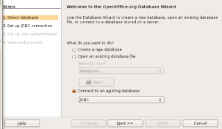
In the 'Set up a connection to a JDBC database' screen I entered

Datasource URL: jdbc:derby:/path/to/Sample
JDBC driver class: org.apache.derby.jdbc.EmbeddedDriver

Clicking on 'Test Class' confirmed the driver was in the Classpath as set earlier. The next screen is 'Set up the user authentication' I leave the 'User name' blank, but check the box labeled 'Password required'

On the next screen, 'Decide how to proceed after saving the database', click 'Yes, register the database for me' which allows OpenOffice.org to access the database (or you just have an odb file that includes database connection parameters) and 'Open the database for editing' ('Create tables using the table wizard' is not useful now since there already are datatables).

OpenOffice.org then asks for a name for the .odb file it will create to maintain the connection to the database (as well as any queries created in OpenOffice.org). The database can be accessed by clicking on any icon ('Tables', 'Queries', 'Forms', 'Reports'). OpenOffice.org will then connect to the database (asking for the database username and password along the way. Entering 'testuser' for username and 'test' for password does it). Then the database can be used from the GUI, which includes a graphical Query Design view or the usual SQL.

Introductory Econometrics with Applications by Ramu Ramanathan

Introductory Econometrics with Applications by Ramu Ramanathan

My review at Goodreads
I've been realizing that most of the data I work with are observational as opposed to the experimental data that most statistics that I know are designed for. So I've been working through this econometrics text. By way of background, I've taken Statistics as undergrad using books and tables, as a master's, which was essentially using SAS, and as a grad student, in a very mathematical sense. Working through Intro. Econometrics with Applications was learning what all the math based stats in grad school, but actually understanding it. And the computer package Gretl makes the learning interactive.

Ramanathan's biggest strength is he does not stop at teaching definitions, formula and methods. And his example applications do not stop at working through methodology. He uses the computer output to build intuition, asking the question of why this variable is what it is, or why two models are different. The use of Gretl enhances this. The scripts and data sets make it easy to see the examples at work, but also make it very easy to explore. I found myself running the scripts, then exploring the data sets in Gretl to further analysis, and building my understanding. The mathematical derivations are there, but having both the theory and the computer outputs for discussion make for a good match.

The book datasets and examples are bundled into the econometrics package Gretl, which is an open source program (available for Windows, Mac, Linux). In addition to correctness (it passes completely the NIST datasets, which is something even SAS and SPSS don't do) the scripts let you see what is happening (as opposed to SAS which often seems like black boxes inside the PROC statement). And more flexible then the menu based packages like Minitab (or Excel based statistical packages). Compared to R/S-Plus there is a shorter learning curve, as Gretl displays more of the output immediately, while allowing various statistics to be exposed for later use if needed (the reverse of R, which exposes statistics, but makes you work to display them. Great for programming, but harder for exploring data to the neophyte.)

I think that texts like this that are integrated with a full fledged statistics package (as opposed to purely math or a demo version) make the learning and applying of statistics different. (other texts that have Gretl datasets available are listed at Data for gretl) The focus of the learning is not on the memorization of equations or definitions, but on the learning of methods and techniques. The chapter summaries become short forms of methodology (as opposed to formula) with the assumptions that the various methods repeated as well. I found this to be a particularly effective format for a first book on a subject (assumes a first sequence in undergrad statistics has been completed).

As of now, I've gone through 5 chapters of the book, working through the examples. As I do this, I am learning a lot about analysis, that is going to inform a project I am starting up. That is probably the best testimony for a book of this type.

View all my reviews.